The split-half reliable path-quadratic score predicted a 16.1% improvement. Complete endpoints then showed that its selected model was 6.0% and 7.7% worse than the two controls. I started this paper from that reversal because it made the problem difficult to dismiss as noisy scoring.
The score repeated. It described the measured path consistently. It still did not contain the information needed to order complete sparse models away from that path. My question became narrower: what decisions can a compression statistic justify from the quantities it actually observes?
Local statistics can propose a small menu. Group-resolved measurements can recover useful structure. The order of complete candidates needs endpoint evidence at the same grain as the decision, and a multistep policy also needs the changing slack to the active worst group.
The score looked reliable
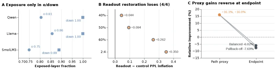
The empirical-Fisher path-quadratic proxy reached 0.906 split-half reliability. In two comparisons it predicted gains of 16.1% and 16.0%. At the complete sparse endpoints, the selected model instead lost by 6.0% and 7.7% against the controls. A stable instrument had produced a stable answer to the wrong decision question.
A fuller Fisher diagnostic helped, but only up to a point. It recovered 7/8 groupwise signs. One predicted 22.1% gain became an inconclusive 2.8% endpoint gain. To me, that is useful local directional information with unresolved endpoint magnitude. It is not a universal selector.
Reliability asks whether repeated measurements agree. Selection asks whether the observed quantities fix the order of the candidates I care about. Those two properties can separate. More calibration samples can tighten a reproducible local estimate without revealing the downstream continuation or off-path values that decide the endpoint.
What a score can actually observe
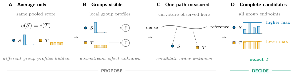
I treat each compression statistic as an information interface. A pooled interface sees an average and discards the supplied group decomposition. A group-local interface keeps the rows for those groups, but still stops at the measured layer. A reference-path interface sees geometry along one declared path. A complete endpoint interface measures every candidate and group used in the actual finite decision.
For one observation, imagine collecting every hidden endpoint table that could have produced it. That collection is the compatibility fiber. If every table in the fiber gives candidate A the same strict order over candidate B, the interface identifies that decision. If two compatible tables reverse the order, no deterministic rule using only that observation can decide correctly in both worlds.
This is an identification result, not a proposal for one universal score. The framework tells me what a declared observation can authorize for a declared candidate family and endpoint. A cheap score may remain excellent for proposing candidates, estimating broad severity, or ruling out obvious failures. Its information boundary says where a new measurement or assumption becomes necessary.
Matched observations can reverse the decision
Matched observations and matched endpoints contain different information. Two admissible models can expose the same pooled moments, the same group-local moments, or the same derivatives along a reference path while assigning opposite orders to two complete candidates. The observation is held fixed. The unobserved continuation changes.
Group-local input evidence still cannot see how an output perturbation propagates through later blocks. Reference-path curvature can be identical to every order along the measured segment while smooth off-path changes alter the candidate endpoints. The score remains internally consistent; its interface has no access to the quantities that moved.
Figure 3 is the empirical version of that construction. Both path-proxy comparisons had strong, repeatable predicted improvements near sixteen percent. Measuring the complete sparse models reversed both decisions. The matched observation therefore supports a proposal, while the matched endpoint settles the comparison.
Broad severity is easier than fine selection
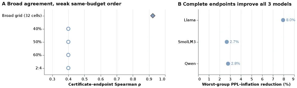
The Llama study crossed two pruning methods, four sparsity settings, and four calibration treatments, producing a 32-condition grid. Across that grid, the group-resolved diagonal tracked realized worst-group damage with Spearman 0.9239. That is strong evidence for broad severity calibration within the declared grid.
Fine same-budget selection was much weaker. The four SparseGPT correlations were all 0.4, with only four treatments at each budget. Group-balanced calibration still improved the broad contrast against pooled C4 by 21.7% for Wanda and 31.5% for SparseGPT. A matched-token Mistral contrast improved by 29.8%. I use those results as calibration evidence, not as a universal ordering over masks at a fixed budget.
I use the split to separate two jobs. Group resolution can tell me that one region of the design grid is broadly safer than another. Neighboring masks still need evidence for their endpoint difference, which depends on compensation, downstream propagation, and the active group.
Complete endpoints rank a finite menu
Dense pruning makes complete measurement manageable by shrinking the search to a declared finite menu. The menu generator's early-preserving allocation improved worst-group perplexity inflation by 20.9% on Llama, 18.3% on SmolLM3, and 12.6% on Qwen against balanced uniform allocation. That coarse depth structure transferred across the three families.
Fine directions remained target specific. Target-matched endpoint measurement improved the declared performance contrast by 7.96% for Llama, 2.68% for SmolLM3, and 2.80% for Qwen. These are finite-menu results. They do not license an unmeasured mask family.
The guarantee stays with the menu. If every candidate-group endpoint has uniform error at
most epsilon and the final aggregator has Lipschitz constant L_psi, minimizing the measured endpoint has at most
2 L_psi epsilon regret on that finite menu. The bound needs simultaneous control
over the whole menu, not a small error bar on the selected candidate alone.
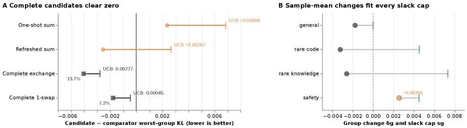
Selection pressure makes that condition visible. In a ten-mask stress test, the winner looked 4.87% better on the selection sample and became 2.76% worse on held-out data. Complete endpoints remove the local transport ambiguity for queried candidates, but noisy reuse of the same sample can still overfit the choice. Independent post-selection data or a uniform menu bound remains necessary.
Router evidence does not rank expert sets
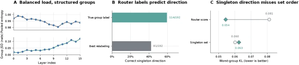
OLMoE exposes group structure directly on removable expert nodes. Its pooled routing load was nearly balanced, with entropy from 0.981 to 0.998, yet 253/1,024 expert-layer cells had group contrast above the declared threshold. The structure repeated cleanly: router mass and routed contribution energy reached split-half Spearman 0.9947 and 0.9832.
Router evidence also helped identify which group would maximize a singleton deletion. Across 192 deletions, it selected the maximizing group in 114/192 cases, compared with 81/192 for the strongest relabeling control. That is useful group visibility attached to the object being removed.
It does not order expert sets. Router traces observe exposure, while the surviving experts' replacement function and later hidden-state changes remain endpoint quantities. Singleton effects can also interact after several experts disappear. I therefore use router evidence to narrow the menu and complete-set queries to decide among the resulting interventions.
Why hard max failed across sixteen layers
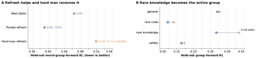
The full-model study removed 25% of the experts from all sixteen routed layers. Pooled endpoint refresh lowered held-out worst-group KL from 0.4647 for the best static score to 0.3912, a 15.8% improvement. Hard max ended at 0.5193, which was 32.7% worse than pooled refresh under matched compute.
The performance endpoint moved differently. Worst-group excess NLL was 0.3157 for static REAP, 0.3655 for pooled refresh, and 0.3764 for hard max. Neither adaptive trajectory improved the performance endpoint. The KL gain is a teacher-coverage result and cannot be promoted into a task or NLL gain.
The group-risk vector explains why greedy hard max failed. A step changes both the current maximum and each group's slack below it. The hard-max trajectory finished close to an active-group boundary, and held-out rare-knowledge risk crossed that boundary. It also changed the menu available at the next layer. One good measured move does not compose into a good terminal policy unless the evolving active face and future candidates remain under control.
What the paper does not establish
The dense evidence covers three main model families, one main sparsity budget, and declared finite menus. The task bridge is one Qwen mask contrast, not a broad behavioral evaluation. Those experiments support the measured endpoint claims within the supplied groups and candidate sets.
The MoE evidence uses one checkpoint and selected one-layer menus.
One sixteen-layer trajectory at 25% deletion completes that evidence.
Adaptive sample reuse entangles path structure and estimation error because later proposals depend on earlier choices made from the same search sample. There is no task-level MoE gain established.
For a new pruning run, I would record the supplied groups, the exact endpoint, and the candidate menu before scoring anything. I would measure the complete finalists, then refresh the group-risk state after an accepted move. Without those records or a validated continuation bound, I would stop at a local proposal claim.